Activities & Plan Management (APM)

Introduction

A primary function of PMRC is tracking recurring activities performed on a daily, weekly and monthly basis. Within the Activities & Plan Management (APM) Module, the user creates monitoring plans that track recurring activities related to either hardware components or commercial activities. The focus of these activities is monitoring process units, crude/products and economic parameters associated to them (yield accounting, margins, prices, costs, etc.). Each activity is configured with one or many parameters. These are the items to be monitored within an activity. They are defined with data such as owner (role), request frequency, monitoring purpose, limits, tolerances, and impact of going over/under limits. In summary, activities configuration information links to the information needed to monitor, including:

• The key performance indicators (KPIs), made of data of different data types such as process variables (ex: reactor temperature profile), pricing, asset status etc.; each of them is a parameter related to the parent activity. They can also be complex processes or studies (ex: backcast result or catalyst activity).
• The target(s) information for each parameter and its data source (ex: operating plan, engineering target, fixed asset constraint).

Components

Components are templates for technical and commercial monitoring activities. Each component can be added to a monitoring plan, and includes preset activities, parameters and targets. Plans are not limited to the items within the component activities list. Components within the "Refinery" section relate to technical monitoring (Process Unit, Catalyst, Reactor, etc.) while those within the "Products" section relate to commercial monitoring. With appropriate permissions, the user can add, edit or delete components. They constitute the company's reference material when it comes to monitoring.

Monitoring Plans

A monitoring plan is a custom set of activities organized in a hierarchy for a specific asset (ex: unit) or commercial entity (ex: Crude oil). Plans are built using a drag-and-drop functionality, so that components can be added and arranged easily.. Each component in the hierarchy represents a monitoring activity or set of activities for process units or commercial functions. When an activity is added to a plan, the associated parameters and targets are included, and can be configured individually. Besides the official "component list" which should be managed as a library (with somewhat restricted access), monitoring plans can be made out of all or some pieces of other monitoring plans.

View & Maintain Component Activities

To view or maintain Component activities, click Configuration > Maintain Component Activities.

Component Hierarchy

The component hierarchy is a list building blocks which can be added to monitoring plans. When an item in the hierarchy is selected, all activities associated with the component are listed in the primary display to the right. Some activities are specific to units. These are listed under "Process Specific." Within this display, authorized users can create, edit or delete components, activities, parameters or targets. Note: Use caution when deleting items. Once they are deleted, they cannot be recovered.

To view the parameters within an activity (or the targets within a parameter), click the arrow beside the activity or parameter.

Edit Component Activities, Parameters & Targets

Click the pencil icon to edit an activity, parameter or target. From this screen, authorized users can edit: asset name, activity name, description, category, frequency, reason, role, priority and comments. Click the Update button to save changes.

Build a Plan

A plan is a custom hierarchy of activities for a specific unit or process. For example, the Process Engineer wants to create a monitor plan for FCCU. He/she creates a new plan by navigating to: Configuration > Create New Monitoring Plan

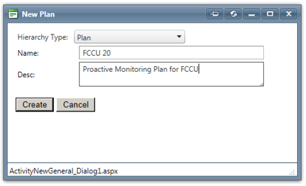
Step 1 - Enter Plan General Information

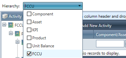
Select a hierarchy type, name the plan and enter a description (ex: Proactive Monitoring Plan for FCCU).

Configure Plan Hierarchy from Components List

Drag/drop items from the component Activities Hierarchy panel to the New Plan Activity Hierarchy, arranging them in the desired order. Adding activities automatically includes the preset parameters and targets, but does not include child components (ex: if "Process Unit" is added to the plan, "Catalyst" and "Separation" are not added).

Note: to hide the left-hand panel, click the arrow to collapse:

After dragging components to the new plan, the user can create, edit or delete activities, parameters and targets. Alternatively, these changes can be performed later, within one of the following three displays: View Plan Activities, Maintain Activities, or Copy Activities displays.

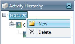
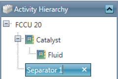
The user can also create new assets / asset categories within the plan hierarchy. To do so, right-click on the desired level within the hierarchy and select "New." Name the asset (for example: Separator 1).

Add activities or drag components to the newly created asset categories. Each item is repeatable - that is, each component or activity can be dragged/added to multiple assets, or added to each asset multiple times and given unique names within the plan.

View & Edit the Plan

To view/edit the plan you created, select Configuration > Maintain Plan Activities, then select the plan from the dropdown list.

Within this display you can add, edit or delete assets, activities, parameters and targets. Right-click to add, rename or delete Assets. Click the pencil icon to edit, or the trash can icon to delete Activities, Parameters or Targets.

Add Additional Components (Copy Activities)

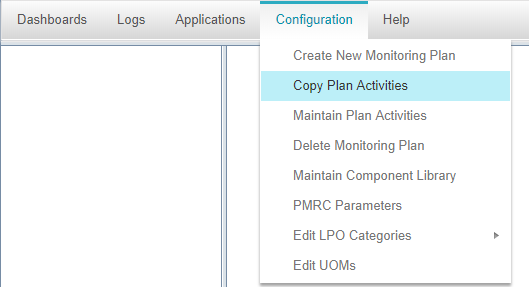
To add additional components after a plan has already been created, navigate to Configuration > Copy Plan Activities

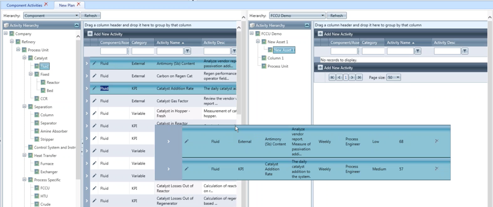
On the left of this display, select the components list, or another hierarchy to drag activities from, then click Refresh. On the right, select the plan which you would like to copy activities to, and click Refresh. You can now drag and drop assets, activities, parameters or targets to the plan.

You can also add multiple activities, parameters or targets at once by holding the control key while selecting the desired items, then dragging them to the asset. First, select the asset to which the activities / parameters / targets will be added. Then select and drag them to the right, as seen below.

Add New Activities, Parameters & Targets

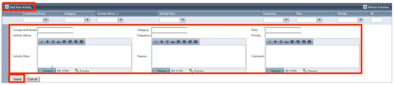
Add Activity: Click the "Add New Activity" button and input details for the component / asset. Click the Insert button to save changes.

Add Parameter: When an activity dropdown button is selected, click the "Add New Param" button and add relevant details. Click the Insert button to save changes.

Add Target: When the parameter drop-down arrow is selected, the user clicks the "Add New Target" button. Input the targets for Lo, LoLo, Hi, HiHi - as well as the causes, effects, and actions for target variances. The target is specific to the parameter in which it is nested. Click the Update button to save changes.

Define Data Source & Function

PMRC currently offers four sources of data for each parameter:

• XL through a template using the parameter ID (in Column A of the sheet) and data column name
• PI through straightforward formula’s similar to XL. PI tags are place between bracket
• PMRC through the following standard views that contain the history of production data - from yield accounting, plans - from LP or schedulers, and prices (custom loads). The data is defined as a simplified SQL query and therefore requires a basic knowledge of SQL (Select, For, Where) - examples can be picked from the existing "Daily Target Sheet" monitoring plan (see appendix) where we have defined both actual production and plan data for a series of process parameters. The views names are:
  • MaterialProductionConsumption: actual fence line charge and production from yield accounting
  • PlanDataMaterial: plan for the above
  • PlanDataProcessUnitMaterial: plan for each process unit
  • ProcessUnitYieldAcctFlow: actual flow in/out of process units - ratable (per day)
  • ProcessUnitYieldAcctMovement actual movements (transfers from/to tanks, from to units) that are not ratable (have a start-time and stop time). Expressed in daily average.
• A predefined SDV (Smart Display and View), which contains all information already (example Charge and Yield Summary, or Indicative Gross Margin). This is only used at the activity level (example monitor material balance) where the SDV name can be mentioned for information (not mandatory). The list of current SDV’s follows. To refer to an SDV, use the URL name without the aspx extension.

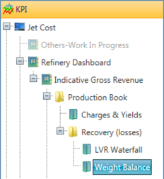
KPI Tree Name	URL
Refinery Dashboard	RefineryDashboard.aspx
Gross Revenue	GrossRevenue.aspx
Production Book	ProductionBookVolume.aspx
Charges & Yields	ChargesYields.aspx
Recovery (losses)	LossRecovery.aspx
LVR Waterfall	LVRWaterfallProcessUnit.aspx
Weight Balance	ProductionBookWeight.aspx
Reconciliation	BackCast.aspx
Monthly Performance Reporting	MPR.aspx
Monthly Production Summary	MonthlyProductionSummary.aspx
Daily Production Summary	DailyProductionSummary.aspx

The following three sources of data can be used for three fields of each parameter:

• The main performance indicator
• An alternate value for the main indicator (from a difference source and/or different time period)
• The "dynamic" target for the main indicator found in the "target" line for each parameter. Note that each parameter can have multiple targets.

Actions / Display Options

Depending on the activity, there are various actions and display options available when the user right-clicks each activity or parameter. The view options allow the data to be analyzed using multiple Smart Views, which dynamically display information for components and commercial activities. Currently these views include:

Target Sheet: a tabular view of each activity of a plan, that displays the three type of data for each parameter (and allows to use trends - see below). Example shown below:

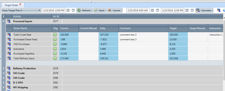
Shown above is the plan called "Daily Target Plan 2" which was designed for daily communication between refinery planners and operations.

We can see each activity (Process Inputs, Refinery Production etc.) with most of them collapsed (Use arrow at left of display), and the first activity expended. This activity lists all its parameters. The three types of data are in the blue columns; in this case: "Current" contains 6-hour average of PI data through formulas (hovering on the formulas would show the PI formula or query result), "Alternate" show 24 hours average of the previous day (from the yield accounting system) and "Target" shows the plan from the linear program.

Columns with white cells are provided for collaboration purpose (standard in all views); it means they can be edited by users and saved. We provide manual override for "Current" and "Target". This would be for instance a way for the scheduler to alter a mid term target (week of month) and change it to a daily target. It also provides columns to enter instructions and to add comments during a collaborative work session. Finally, by hitting the person symbol, the user can access a registry to enter a Lost Profit Opportunity or an Action Item. All these fields can be saved through one command at the top.

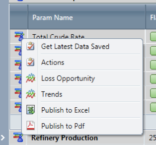
The same menu allows retrieving the last data saved in case the user wants to start anew.

Rolling to a new day can be done through to commands on the top of the screen:

The user can select the monitoring plan (here "daily Target Plan 2"), pick an operating day, pull data from the database, save, cancel, adjust the time period within the operating day (this would impact the "function" defined in each parameter if applicable - example: Average). Upon pressing Calculate, all data would be retrieved automatically for the operating day and period. Make sure to save prior in case you want to roll comments, targets and instructions to the new day.

Publishing to Excel or PDF is also available from the tool tip on the right.

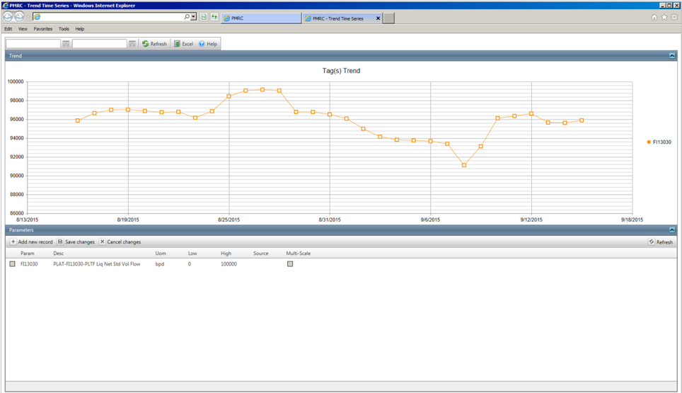
Trends: Right-click and select "Trend" option to display each of the activities and parameters trend graphs; these trends can also be available from the View Activities and in relevant SDV’s such as the Engineering Display."

Example Queries

General Examples

Statements mirror SQL without need to enter Select, For, Where.

Start with [ then Q:

Open Select {

End of Select }

Open Where {

End of Where }

() used for formulas within statement

Use of PMRCXP table names (see section 4.3) and yield accounting naming convention (taken as PMRC master) and Product Master List with Materialtype, MaterialSubype and MaterialName (also taken from yield accounting master)

Other attributes and functions:

OperatingDay: the day period for the query

DateAdd: add or subtract days to operating day

UOM such as BarrelsperDay to change display of UOM defined in the parameter.

Specific Examples

• Get Crude charge to refinery from PMRC for previous day:
  [Q:{SUM(ClosingInventory - OpeningInventory + ShipmentsNetVol - ReceiptsNetVol)}{MaterialProductionConsumption}{MaterialSubtype like '%Crude%' and OperatingDay = DATEADD(DAY,-1,%OPERATINGDAY%)}]*-1
• Get gasoline production - components and finished product from PMRC for previous day:
  [Q:{SUM(ClosingInventory - OpeningInventory + ShipmentsNetVol - ReceiptsNetVol)}{MaterialProductionConsumption}{(MaterialSubtype like '%Gasoline Blendstocks%' or MaterialSubtype like '%Motor Gasoline%') and OperatingDay = DATEADD(DAY,-1,%OPERATINGDAY%)}]
  
• Get Plan for gasoline and gasoline production components form PMRC:
  [Q:{SUM(PlanDataMaterial.BarrelsPerDay)}{PlanDataMaterial}{PlanDataMaterial.YieldAcctMaterialName like  '%Gasoline Blendstocks%' or PlanDataMaterial.YieldAcctMaterialName subtype like '%Motor Gasoline%''and OperatingDay = DATEADD(DAY,0,%OPERATINGDAY%)}]
  
• Get Jet A plan from PMRC:
  [Q:{SUM(PlanDataMaterial.BarrelsPerDay)}{PlanDataMaterial}{PlanDataMaterial.YieldAcctMaterialName = 'JETA'and OperatingDay = DATEADD(DAY,-0,%OPERATINGDAY%)}]
  
• Get CDU543 charge for yesterday from PMRC:
  [Q:{SUM(isnull(RecLiqNetStdVolFlow,LIqNetStdVolFlow))}{ProcessUnitYieldAcctFlow}{DestNode = 'CDU543' and OperatingDay = DATEADD(DAY,-1,%OPERATINGDAY%)}]
  
• Get total crude charge plan from PMRC:
  [Q:{SUM(PlanDataProcessUnitMaterial.BarrelsPerDay)}{ PlanDataProcessUnitMaterial,Materials, MaterialTypes}{PlanDataProcessUnitMateriall.YieldAcctMaterialName = Materials.Name and Materials.MaterialType_Id = MaterialTypes.Id and MaterialTypes.Name like '%Crude%' and ProductionConsumptionFlag='C' and OperatingDay = DATEADD(DAY,-0,%OPERATINGDAY%)}] * -1
  
• Get CDU 543 planned charge from PMRC:
  [Q:{SUM(BarrelsPerDay) * -1}{PlanDataProcessUnitMaterial}{YieldAcctUnitName='CDU543' and MaterialSubType like '%Crude%' and OperatingDay=%OPERATINGDAY%}]
  
• Get All FCC charge for yesterday from PMRC:
  [Q:{SUM(isnull(RecLiqNetStdVolFlow,LIqNetStdVolFlow))}{ProcessUnitYieldAcctFlow}{DestNode = 'FCC' and OperatingDay = DATEADD(DAY,-1,%OPERATINGDAY%)}]
  
• Get Reduced Crude rate to FCC for yesterday:
  [Q:{SUM(isnull(RecLiqNetStdVolFlow,LIqNetStdVolFlow))}{ProcessUnitYieldAcctFlow}{DestNode = 'FCC' and SourceMaterial like '%CRSD' and OperatingDay = DATEADD(DAY,-1,%OPERATINGDAY%)}]

Review Unit Balance

Introduction

Performance Monitoring and Reporting Center includes a module called CLN (Collaboration, Logs & Notifications) where the Process Engineers can use the Review Unit Balance display to monitor the process unit balances and send feedback to yield accounting.

Each user can monitor the material balance of units allocated to him/her using PMRC. However, all engineers will be able to see all units configured in S-TMS (the yield accounting system) and they will be displayed under the "Process" node in the tree view on the left panel. If an additional unit/node is setup in S-TMS, it will be displayed in the left panel. By default, the data displayed when PMRC is opened is the data from the previous day. As mentioned above, Engineers can access any unit but are expected to make modifications to their assigned units only.

The data within PMRC can contain raw, compensated (corrected for actual temperature, pressure and gravity) and reconciled balance data; the reconciled data only appears when movements around the process unit are reconciled by Yield Accounting (in S-TMS); it replaces the compensated data (it is a higher quality data). There are cases where the raw flow data is not available because the stream is not metered or the meter is faulty. In these cases, until the reconciliation is performed, the stream (raw and compensated) will display as 0 where there is no meter and the balance will be affected accordingly. The reconciled values will appear once reconciliation is done.

Access Review Unit Balance

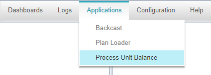
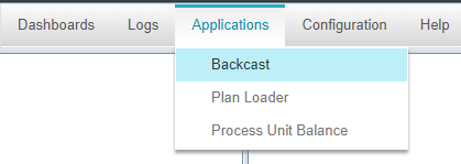
From the PMRC main menu, access to the Review Unit Balance display by clicking Applications -> Process Unit Balance as shown in the figure below:

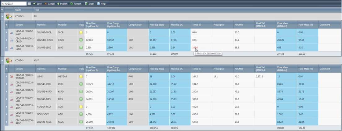
Review Unit Balance Display

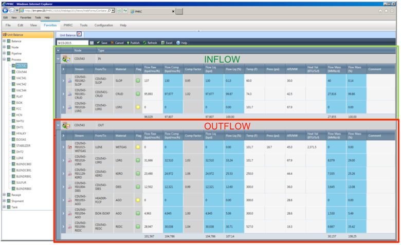
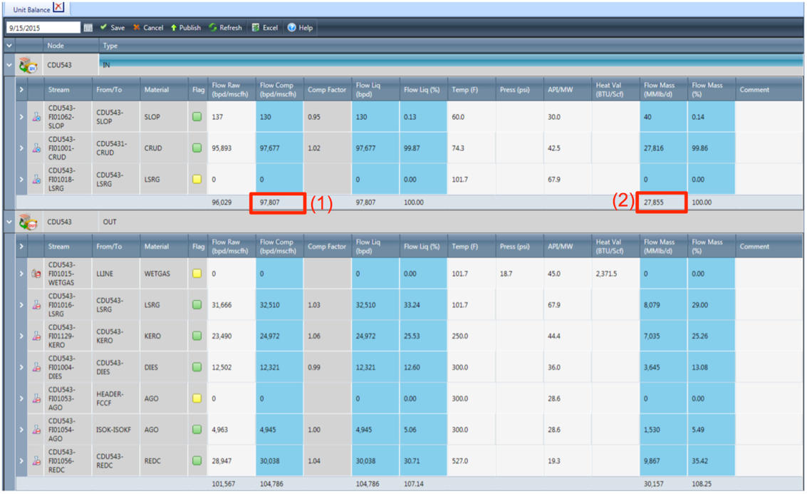
Select the unit that you want to review in the left panel. When the unit balance displays in the main window, the top portion of the screen shows the unit Inflow grid (indicated by type: IN), and the bottom portion of the screen shows the unit Outflow grid (indicated by type: OUT).
Columns highlighted in blue are calculated values. White columns are raw data from PI, and can be edited by the end-user. Grey columns are read-only data.
From the unit balance tool bar, the user can perform the following actions:

• Click on the Date button or enter a date in the selection field. When you have selected a date, the data in the grid will automatically refresh.
• Click the Save button to save the modified data to the database with status "Pending" for later use without sending an email to the Yield Accountant.
• Click on the Cancel button to cancel all changes made to the raw values.
• Click on the Publish button to save the modified data to the database with status "Published" and send an email to the Yield Accountant indicating that changes have been made to the raw data.
• Click on the refresh button to refresh the grid with data from the database.
• Click the Excel button to export the data as a spreadsheet. When the save dialog appears, choose the option to save as, then select the location and open the file from your local computer. When the file is downloaded and opened, Excel warns that the file format is different than the specified extension. Please ignore the message and click "Yes" to open the file.
• To view the data trend, right-click on the specific cell/value and select Show Trend. A new tab opens, displaying the data as a trended graph. The default date range shows the previous month. The source of the data trended is from S-TMS.

The following figure shows the different sections of the Review Unit Balance display:

Default Data Column Descriptions

See the image below to view the data and columns defined in this section.

• Inflow Rate Key Total - The total flow rate used to calculate percentages for both in & out streams. The inflow rate key total is shown below the compensated flow column
• Inflow Mass Key Total - The total flow mass used to calculate percentages for both in & out streams. The inflow mass key total is shown below the compensated mass column
• Stream - Displays each individual stream ID to and from the unit. Icons in the column to the left indicate:
  • It is a liquid stream (denoted as a beaker)
  • It is a gas stream (denoted as a gas tank)
  • It is an inflow (denoted by blue IN badge)
  • It is an outflow (denoted by red OUT badge)
• From/To - Where is the material flowing from/to (S-TMS nomenclature)
• Material - Material to/from unit
  • Hover over the material to view the full material name; also picked up from S-TMS
• Flag - Status indicator
  • Green indicates normal operation
  • Yellow indicates the data is 0, or the compensated factor is +/- 10% difference
• Flow Raw - Raw flow data from PI or manual entry by accountant
• Flow Comp - Compensated flow based on actual flowing temperature, pressure, and actual gravity in standard conditions.
• Comp Factor - The compensated flow divided by the raw flow
• Flow Liq (bpd) - Compensated liquid flow where gas streams are converted in FOEB
• Flow Liq (%) - Percent of liquid based on the inflow rate key total
  • NOTE: Flow Liq (%) also based on inflow key total
    • The inflow key total is used to calculate output percentages; note that this is slightly different from a pure LVR calculation where liquid outflows percentages are based only on total liquid input and not on total input (liquid and gas in FOEB)
• Temp (F) - Raw temperature data from PI in degrees Fahrenheit
• Press (psi) - Raw data from PI. Only used on gas
• API/MW - Raw density / molecular weight (API for liquid, and MW for gas)
• Heat Value (BTU/Scf) - Raw data for gas only
• Flow Mass (MMlb/d) - Mass in million pounds per day, calculated by a formula in S-TMS
• Flow Mass (%) - Based on key inflow mass key total

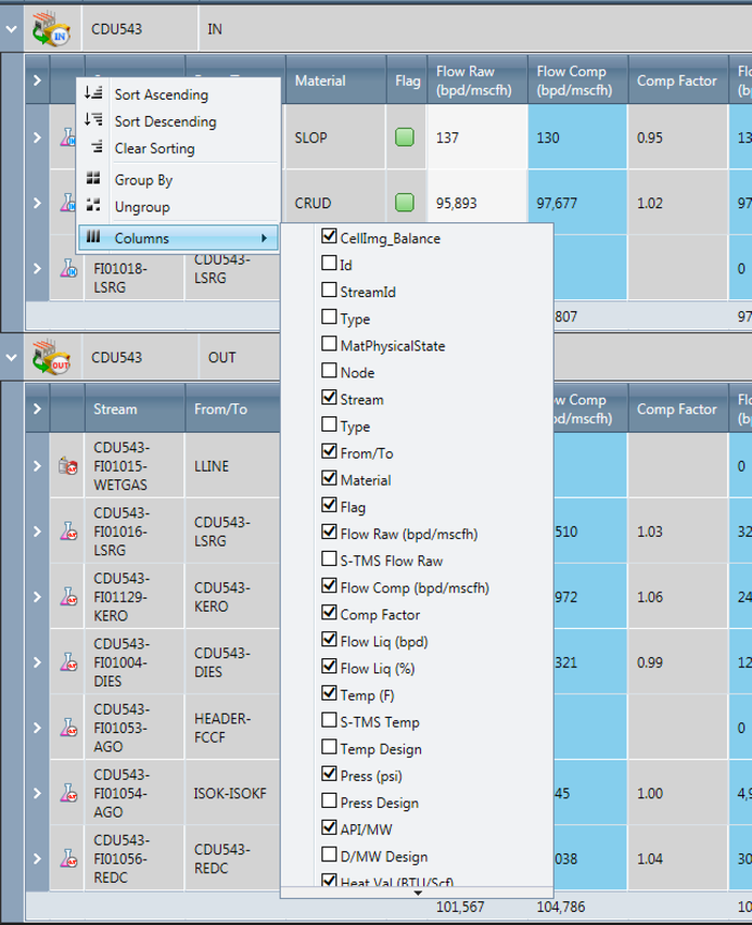
Additional Columns

Additional columns can be added to the view in PMRC, such as the ones displaying S-TMS configuration data for gravity, temperature and pressure . To add columns to the inflow and outflow areas, right-click the column heading area, and hover over Columns. Select the check-boxes of the columns you would like to add to the view. This view change affects the inflow and outflow grids separately. That is, if you would like to add specific columns to both grids, they must be selected separately. When you add columns, the view settings are used as the default for that user.

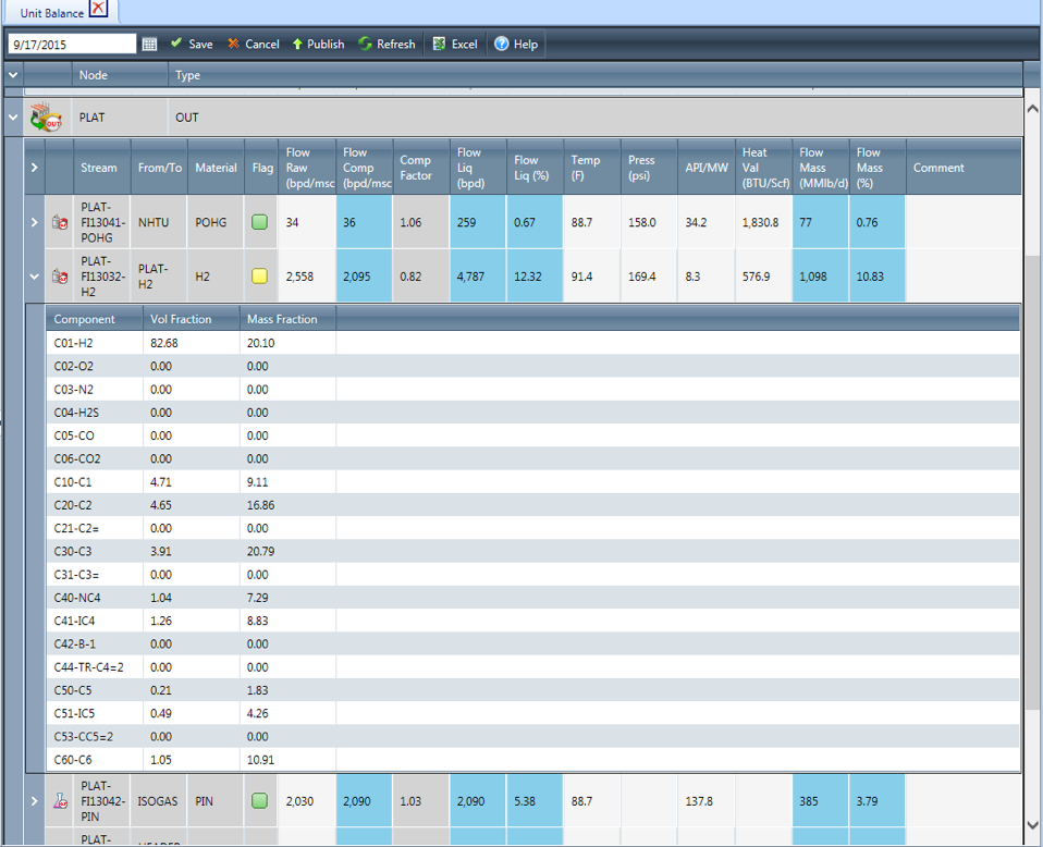
Gas Composition Data

To show the gas composition of a specific gas stream, click on the Expand/Collapse button at the beginning of each stream row in the grid. If the stream is associated to a gas and the composition data is available, the display will show the volume and mass factions of each component associated to the gas, as shown in the following figure:

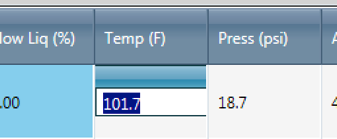
Edit Data

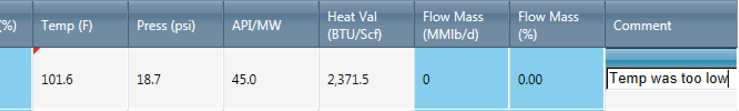
To edit any of the raw PI data (cells with white background), double click the cell, enter the new value and press Enter. When the data is edited, the cell is flagged with a red triangle in the upper-left corner. The user can enter a comment in the Comment field, to specify the reason for the change.

When you press Save, it saves the changes to the database but doesn’t alert the Yield Accountant. When you press Publish, the system sends an email to the Yield Accountant to alert them of the change(s).

When the change is published, the red flag within the cell is no longer displayed, but the edited value in the cell is shown in a red font color.

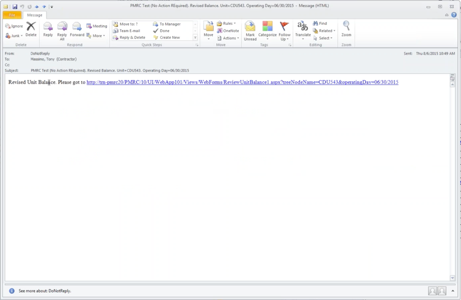
Data Change Alert Email

When data changes are published, the Yield Accountant receives an email to alert them of the change. The subject line specifies what changed, on which unit, when the change was made and who made the change. Clicking the link doesn’t open the full PMRC interface, but rather opens the data screen which displays what changed. Hovering over the changed data field reveals the original value in S-TMS.

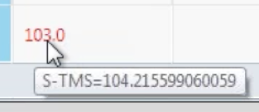
Above: Hovering over the red (edited value) shows the original value.

View Trends

To view the data trend, right-click on the specific cell/value and select Show Trend.

A new tab opens, displaying the data as a trended graph (fig.8). The default date range shows the previous month. The source of trended data is from the S-TMS database.

Export Data to Excel

Click the export to Excel button to export the data. When the save dialog appears, choose the option to save as, then select the location and open the file from your local computer.

When the data is downloaded as Excel, PMRC creates an XML file with an XLS file extension. Therefore, when the file is downloaded and opened, Excel warns that the user that file format is different than the specified extension. Click "Yes" to open the file.

Profit & Loss KPIs

Introduction

A primary function of PMRC is tracking refinery performance using the Key Performance Indicators (KPIs) to display commercial and operational performance trends. The Smart Dashboards & Views module allows the user to examine revenue and production data against plans and targets for specified date ranges in a variety of views and graphs. The KPIs also compile and calculate the monthly production data to present the Monthly Performance Report.. This data can be displayed at the high-level, in the Refinery Dashboard, or accessed in more detail within the production book (Charges & Yields) for each process unit or product.

To access the Profit & Loss KPIs module, navigate to:
Dashboards > Profit & Loss KPIs

Refinery Dashboard

The Refinery Dashboard displays graphs of overall performance data for the refinery. Specify the date range in the date selection box and click the Refresh button.

Dashboard Graphs & Data

The Refinery Dashboard includes the following data in graphs and tables:

• LPOs (Lost Profit Opportunities) per Category: operational, mechanical or commercial; displayed as a pie graph.
• LPOs per type, caused for example, by: product downgrades, octane giveaway, slop re-run or volatility giveaway; displayed as a pie graph.
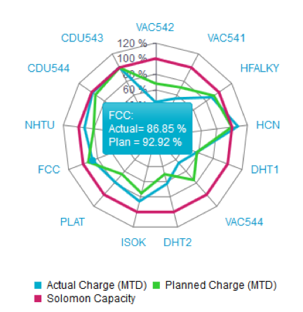
• Actual vs. plan feed/product rate; displayed as a spider graph, showing actual and plan percentage of utilization of each unit versus the Solomon capacity. By clicking on a process unit’s name, the charges and yields dashboard will be displayed.

• Monthly production: actual vs. planned production per product family; displayed in a bar graph.
• The summary table displays daily and month-to-date actual versus planned values. The daily value is from the last day in the selected period. The following categories are included in the table:
• Refinery Crude Rate: the crude charge, listed by crude type in the Crude Slate
• Intermediates Feed Rate
• White Products
• Jet Fuel Production
• Crack Spread: Gross revenue per barrel
• Liquid Recovery (sum of all liquid products as % of liquid feed to the refinery)

Heat Map

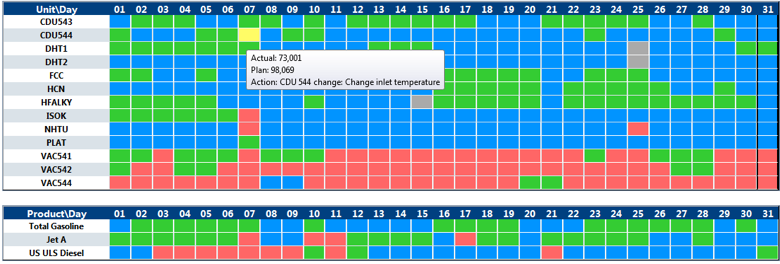
The heat map at the bottom of the screen displays daily performance by unit/date and by product/date combinations. Color blocks that represent the unit status indicate results for the selected period:

• Blue: Actual value is more than planned value
• Green: Value is within 20% of planned production
• Red: Value is below 20% of planned production
• Yellow: The issue affecting production has been identified and an action has been logged in the system. There is an LPO and an action item for this day and unit.
• Gray: No data for that unit/day in S-TMS or the unit is offline

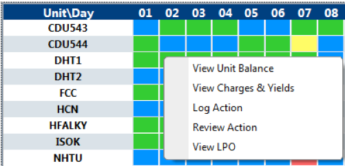
Process Unit Heat Map Options

From the process unit heat map, the user can right-click a unit/day to:

• Review the unit balance data - detailed balance by volume and by weight daily and month to date
• View charges and yields - summary charges and products compared to plan
• Log an action; review an action
• View lost profit opportunities associated with the unit

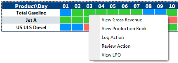
Product Heat Map Options

From the product heat map, the user can right-click a product/day to:

• View gross revenue dashboard
• View the production book
• Log an action
• Review an action
• View lost profit opportunities associated with the product

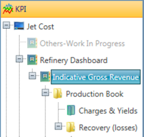
Indicative Gross Revenue

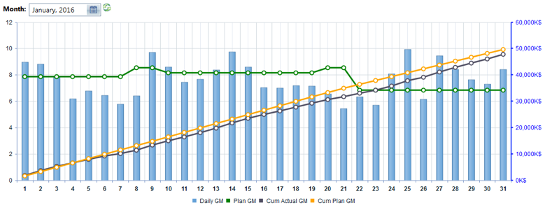
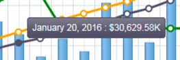
Gross Margin Graph

Navigate to the left menu within the Refinery Dashboard tree and select the Indicative Gross Revenue menu item. Select the month to review in the date selection box at the top right then click the "OK" button.

The blue bars in the graph represent the gross margin in dollars per barrel for each day in the period. These margins are "indicative" in the sense that they use market prices produced by Atlanta’s optimization group, and not the final sales prices or purchase costs. The green line represents the Planned Gross Margins, which are loaded into PMRC every month . The purple line on the graph represents the Cumulative Actual Gross Margin. The orange line represents the Cumulative Plan Gross Margin. Hovering the mouse cursor over any of the bars or points on the graph will display the gross margin value. The data in this graph is calculated from the details shown in the Feedstocks and Products tables below.

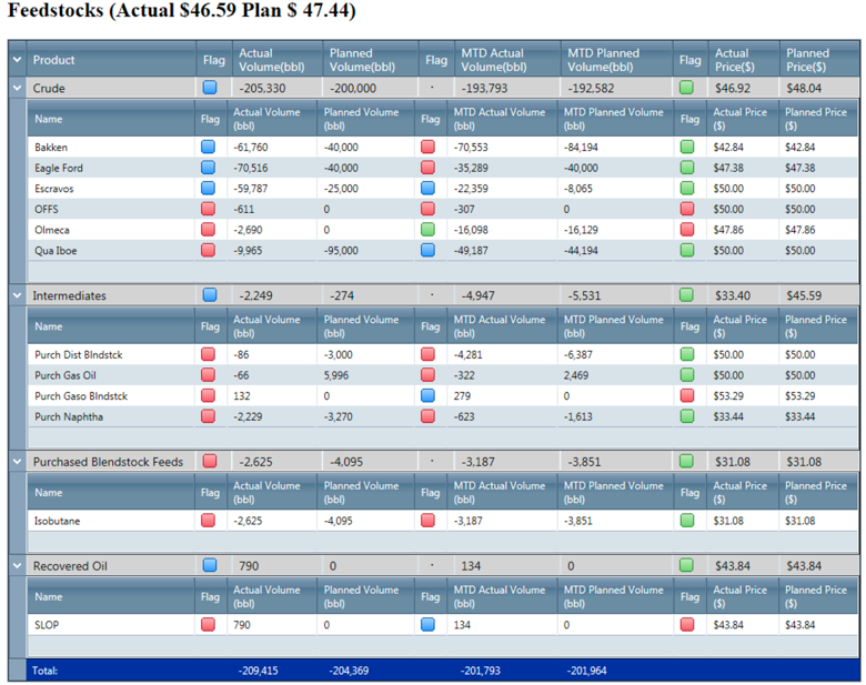
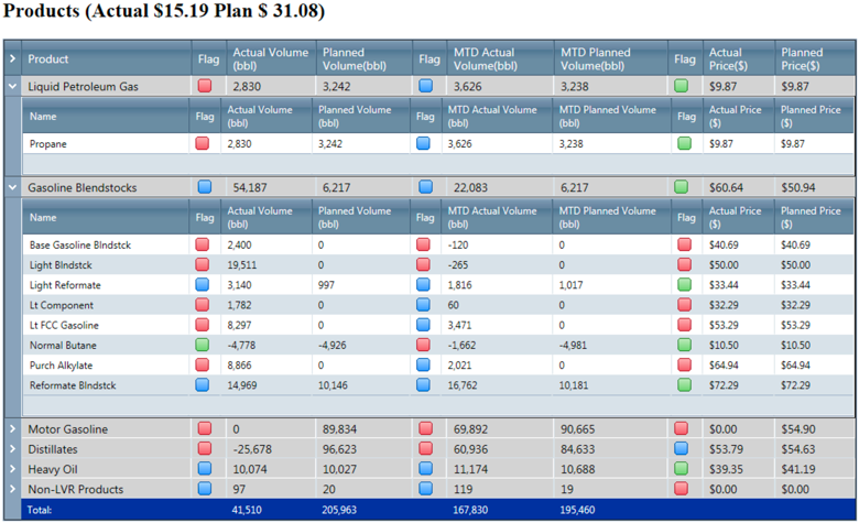
Actual vs. Plan Table

The data in the Actual vs. Plan table is shown visually in the Gross Margin Revenue graph discussed in the previous section. The data for the plan is loaded into PMRC from LP outputs (requires Atlanta to send the new files), and the actual production data is imported to PMRC by an automated feed from S-TMS. Each feedstock and product family contains a nested list of commodity types. To view the nested feedstocks/products click the arrow button. The charge volume is shown as negative numbers (consumption), and yield volume is shown as positive numbers (production) - this is a universal rule within PMRC: negative volume is a charge (disappears in processing), and positive is a product (created in the process units and blends). The table displays daily actual vs. plan volumes, month-to-date actual vs. plan volumes, actual vs. plan prices, and performance indicator flags. Product prices are automatically imported to PMRC from the source Excel workbook maintained by the commercial operations team in Atlanta.

Performance Indicator Flags

The performance indicator flags in these tables use the following colors to correspond with each value:

• Blue: value is above planned production
• Green: value is within 5% of planned production
• Yellow: value is within 10% of planned production
• Red: value is more than 10% variance from planned production

For raw material cost, lower than plan is good (blue) and higher than plan is bad (yellow/red). For products, higher than plan is good (blue) and lower than plan is bad (yellow/red). In the case of negative production (inventory down), we do not include the price in the weighted average of a category (example: gasoline blend stocks) because it can create distortions in results.

Production Book

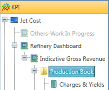
To view the detailed production data within the Production Book, navigate to: Refinery Dashboard > Indicative Gross Revenue > Production Book

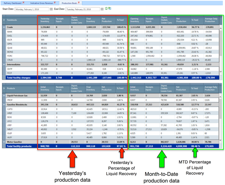
Specify the date range and click the Refresh button.
The primary production book displays values in volume (barrels). There are two tables: one for feedstocks and the other for finished products, with nested feedstock and product families. The left half of the table displays yesterday’s production data (from left to right): Starting Inventory, Receipts / Inputs, Shipments, Final Inventory, Net Production, and Percentage of Feedstock used.
The right half of the table displays month-to-date production data (from left to right): Opening Inventory, Receipts / Inputs, Shipments, Final Inventory, Net Production, Percentage of Feedstock used, and Average Daily Production.

Production Book by Weight

To view the production data by weight, navigate to the Weight Balance menu item within: Refinery Dashboard > Indicative Gross Revenue > Production Book > Recovery (losses) > Weight Balance

Specify the date range for the production data then click the Refresh button. The weight balance includes non-LVR material such as Coke, Sulfur and Fuel Gas.

Charges & Yields

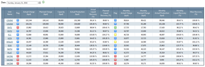
There is one line per process unit with summary information for the selected day as well as month to date data. The flags represent variance to plans both for the daily values and for the month to date values. Color codes are as before: bleu: higher than plan; green: within 5%, yellow: within 10%, red: less than 10% of plan
By clicking on a specific process unit, the detailed balance will be displayed (shown below).

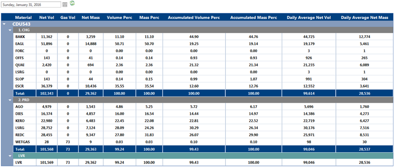
This balance is coming from the yield accounting system STMS; it shows the best available data, so it would use reconciled values if they exist, if not, it uses compensated flow values. The reconciliation allows calculating a composition of the crude charge to each crude unit. Therefore, seeing a generic crude (CRUD) in the daily volume would indicate that reconciliation was not run that day, or not exported (export is a function triggered at the STMS level in order to move data rom STMS to PMRC). If the generic CRUD code is in the month to date column and not in the Daily column, it means that at least one day prior to the selected date was not reconciled or exported. These issues can be corrected by contacting the yield accounting department.

Recovery & Losses

Specify the date range then click the Refresh button. To view data for the entire month, select the last day of the month.

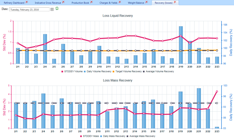
The graphs above display the daily liquid and mass recovery (loss) percentages, including standard deviation, target recovery and average recovery. The standard deviation is calculated over the last 10 days, e.g., the standard deviation for February 1 is calculated from the average deviation for values for January 22 - 31. The target volume recovery is calculated from the plan (total liquid product/total liquid feed). The target weight recovery is set at a fixed 100%, there fore not displayed
By clicking on a liquid recovery column, the volume production book of the selected day will be displayed.
By clicking on a mass recovery column, the weight production book of the selected day will be displayed.

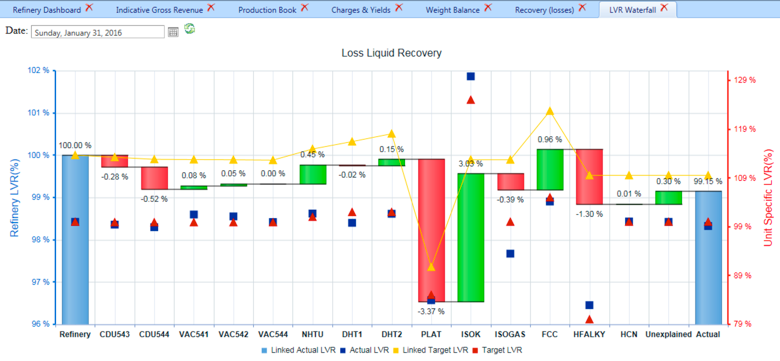
Liquid Volume Recovery Waterfall

To access the LVR Waterfall display, navigate to: Refinery Dashboard > Indicative Gross Revenue > Production Book > Recovery (losses) > LVR Waterfall

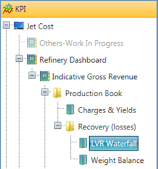
In this waterfall graph, the liquid volume recovery is displayed for each process unit. When the user hovers the mouse over each component, more information is displayed regarding liquid volume gains and losses. The individual points (blue square and red triangle), represent the actual vs. target LVR for the unit (total liquid product/total liquid feed). While the connected points, and the bar graphs, show volume as percentage of total feed to the refinery. The concept is that the refinery starts with 100% volume in the crude tanks, and then some volume amount is lost or gained through each unit, leading to the volume recovery indicated in the production book for that period. The target unit recoveries can be updated in the monthly performance set up table (see MPR). The diagram realistically requires for the unit to be weight balanced to 100%, which is the case when full refinery reconciliation is performed. In order to produce a decent set of intermediate data in case the refinery is not fully reconciled, we are normalizing the yields to a sum of 100% weight. The unexplained bar (first bar left of "Actual") is the gap between LVR actual and cumulated LVR after going through reported units.

Material Allocation

To access the Reconciliation display, navigate to: Dashboards > Profit & Loss KPIs > Refinery Dashboard > Indicative Gross Revenue > Material Allocation
Material Allocation presents another view of how well tank-to-tank balance (Fence Line - A) matches internal transfer to/from process units and intermediate movements between tanks (Refinery Transfers - B).
Material Allocation is displayed in two tables: one for feedstock, and one for products (including intermediates if they have storage capacity). The view displays data for the selected day, as well as the month to date information. At the summary line is the difference of volume consumption or production calculated from the fence-line perspective (inventory change + shipment - receipts) or the transfer perspective (all other transfers inside the refinery).
By expending each product, the user has insight of where the production came from. For example: one can see where low sulfur distillate came from (from the bottom of hydrotreaters and other sources). The table can be exported to Excel by pressing the Export to Excel button at the upper left section of the display.

Monthly Performance Report (MPR)

The Monthly Performance Report displays detailed production data, highlighting areas of concern and opportunities for improvement. The report is configured to emphasize common stress points for production, utilization, reliability, lost profit opportunities, giveaways, blends, etc. It mirrors the information presented at the monthly performance review meeting (MPR). To access the Monthly Performance Reporting display, navigate to: Refinery Dashboard > Monthly Performance Reporting. When the display opens click the calendar icon and select the desired period. Click "OK" and then select the Refresh button. At the end of each month, the user will click the "Calculate" button to update all values in the MPR. There is also a collapse and expend all button at the top of the screen as well as a capability to expend or collapse one section at a time. This is useful for on line presentations

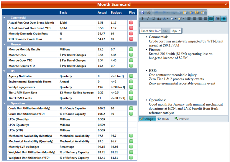
Month Scorecard

The Monthly Scorecard tracks the production data from automated feeds along with the user provided plan / activities to display a high-level view of how the refinery is performing against the plan. In order to enter some data manually, The user has created a plan in the APM (Activities & Plan Management) module: the monthly performance plan; In the viewing mode (PMRC Menu/Actual versus Plans/Monthly Performance Reporting, the user enters a few additional values associated with actual performance and target from the finance and HSE systems. The metrics include performance data for Commercial, Finance, HSE and Operations.
Metrics that are provided by the user in the APM module include:

• HSE
• Mechanical Availability
• Operating Expense (Opex): Monthly & YTD
• Monroe Results: Monthly & YTD
• Monthly LVR vs. Budget

Metrics that are calculated by PMRC using the plan and automated data feeds include:

• Domestic Crude Runs: Monthly & YTD - from STMS data
• Crude Unit Utilization: Monthly & YTD - from STMS and budget data
• LPOs: Monthly, Quarterly & YTD - from the LPO module
• Weighted Unit Utilization: Monthly & YTD - from STMS and budget data

The values are displayed in the table within four columns: basis, actual, budget and flags. The actual and budget are compared, and if the actual deviates from the budget (conditionally, above or below), a simple alert flag is displayed (red versus green). For example, if the actual run cost over Brent is higher than the budgeted run cost, the system displays a red status flag. Or if the actual number of health or safety events is more than the budgeted amount the red status flag will be displayed. These rules can eventually be edited to include more conditions and colors.

Comments

For each section in the MPR, the user can enter comments relating to the performance data. When comments are saved, all PMRC users will see them in the system.

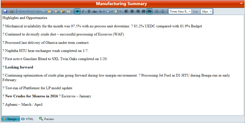
Manufacturing Summary

In this section, the user enters any additional comments related to manufacturing performance for the selected month.

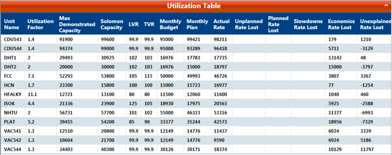
Utilization Table

The utilization table displays a summary of production data for each unit per month. The values in this table are used to calculate the data for the Monthly Reliability and Utilization bar graph below. The Actual Rate values are calculated within S-TMS. The user provides the following values (configured at the beginning of the year):

• Utilization Factor
• Max Demonstrated Capacity
• Solomon Capacity
• Liquid Volume Recovery (LVR)
• Total Volume Recovery (TVR)
• Monthly Budget
• Monthly Plan (updated periodically by user)

The user enters the LPO values in the LPO Summary Dashboard, including start time and end time. From the LPO Summary, PMRC calculates:

• Unplanned Rate Lost
• Planned Rate Lost
• Slowdowns Rate Lost
• Economics Rate Lost (difference between Solomon Capacity and the Monthly Plan)
• Unexplained Rate Lost

LPO Summary Dashboard

For each lost opportunity, the user will navigate to the LPO Dashboard to enter the details of the event. To access the LPO Dashboard, navigate to: Logs > Lost Profit Opportunity (LPO)
The user logs the details for each lost opportunity using the drop-down menu, date selector or text entry, and include:

• Origin - from pick list (Commercial, External, Logistics, Mechanical, Operational)
• Type - from pick list (Demurrage, Production Loss, Product Downgrade, Volatility Giveaway, Octane Giveaway, etc.)
• Event - user entry (example: Average giveaway for the month, slop rerun, etc.)
• Start & End Time
• Equipment - from pick list
• Product - from pick list
• Quantity - optional but recommended for "unplanned outage", "planned outage", "giveaway" and "production slowdown"
• UOM (Unit of Measure)
• Quality - as needed for give away
• Dollar/Unit - as needed for giveaway
• Dollar Estimate
• Dollar Manual - mandatory if it is to be included in the MPR report.
• Root Cause - from pick list (Catalyst, Crude Quality, Containment, Leak, etc.)
• Comment

Origin, Type and Root Cause pick lists are prepopulated with items used in reports until 2015. Equipment and Product pick lists are taken from STMS.

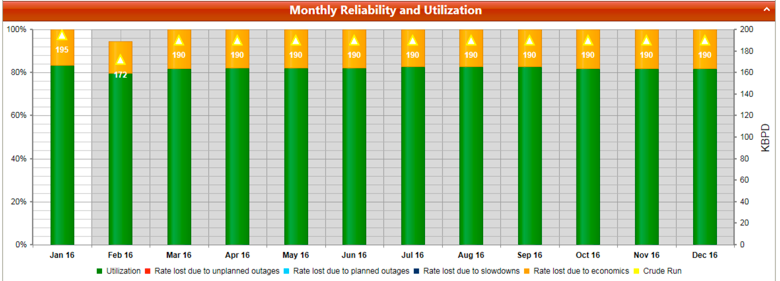
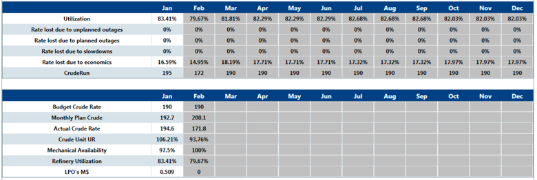
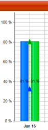
Monthly Reliability and Utilization

This graph is a visual representation of monthly utilization values, including percentages of rate lost and the underlying causes. It uses the LPO registry to consolidate the barrels lost by type. The barrels lost due to economics are calculated as the difference between the plan unit throughput and Solomon capacity The first table below displays the percentages of rate loss and underlying causes. The second table displays numbers and percentages for the following:

• Budget Crude Rate
• Monthly Plan Crude Rate
• Actual Crude Rate
• Crude Unit Utilization Rate
• Mechanical Availability
• Refinery Optimization
• LPOs (in M$)

Product Capacity

For each month, the given capacity for Gas and Diesel is compared to actual production, and shown in the graph as Actual Percentage of Capacity versus Planned Percentage of Capacity. The blue bars represent actual percent of capacity and the green represents plan actual percentage of capacity.

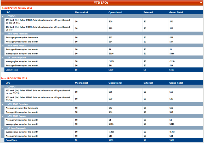
YTD LPO

In these two tables, lost profit opportunities are displayed in thousands of dollars: In the first table, the selected period is shown; in the second table, the year-to-date is shown. This graph is comprised of LPO data provided by the user in the LPO Summary Dashboard, described in section 7.3.1.

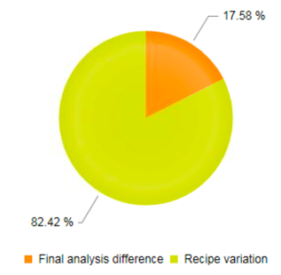
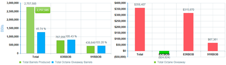
Gasoline Octane Giveaway

The graphs and tables in this section display the root causes of octane giveaway, which are input by the user in the LPO Summary Dashboard. The giveaway is logged as quality differential above or below target. The pie graph displays the percentage of root cause for octane giveaway.

The bar graph to the left displays the barrels produced in green, and the octane giveaway barrels in blue. The bar graph to the right displays total octane giveaway in dollar amount. Where there are negative octane giveaways, a gain is shown, as is the case for 83CBOB.

Gasoline Volatility Giveaway

This section is structured similarly to octane giveaway, but specific to volatility giveaway. Displayed at the bottom of this section is the total octane giveaway (green) and volatility giveaway (blue) in barrels.

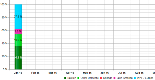
Crude Blend

The bar graph in the Crude Blend section displays various categories of crudes run in each month.

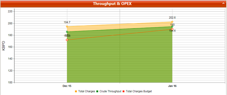
Throughput & OPEX

For each run, the graph in this section displays: total crude charge, crude throughput and total charge budget.

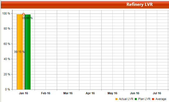
Refinery LVR

The graph at the top of this section displays actual LVR (yellow) versus the planned LVR, and the average is shown in the line on the graph.

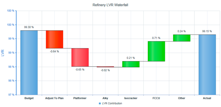
Refinery LVR Waterfall

The waterfall graph in this section is calculated using the refinery budget value as the basis, rather than 100% basis, as used in the Recovery (Losses) LVR waterfall. This graph includes adjustments to the plan, and focuses on big LVR contribution units: Platformer, Alky, Isocracker, and FCCU. The "Other" column shows total unexplained loss. The actual column shows the total volume recovery of the refinery. This graphs data is currently entered manually.

Production Summary

Monthly Production Summary

This report is similar to the production book; it displays all products and feedstocks with final production numbers. Select the start and end date, and click refresh. Each production month in the selected period is shown, with the month listed in the column heading.

Daily Production Summary

Displays the production book for each day in the selected month.

Backcast

Backcast is a small application that allows to produce a reconciled material balance by volume (STMS creates a reconciliation by weight), and to load up to three LP case outputs into PMRC. Reports are then generated to compare the actual volume reconciled performance to each LP case output. All reports can be exported to Excel at once. Backcast is accessed through Favorites.

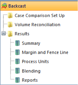
The Menu is then displayed on the left side of the screen and mimics the process of backcast (collect data, reconcile by volume, run and load case, set up cases, generate reports).

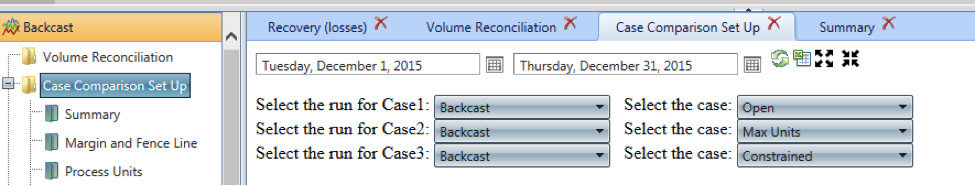
Case Comparison Setup

The Backcast application gathers actual production data for a period of the past to be studied (typically a calendar month), and compares the data to the output of three linear programming (LP) cases. These cases, called Case 1, Case 2 and Case 3, represent the optimum output from the LP setup in actual conditions of the month being studied, but in a gradually more restricted set of variables (from Case 1 to Case 3). It uses Actual prices for the month studied -- typically market-based prices for the location, and the comparison is therefore made at the gross operating margin level (product value -- feedstock cost -- variable costs such as utilities and chemicals). Case 3 is configured to be the nearest representation of actual production, and therefore can also generate a list of improvements for the LP. The other cases complement the study (each company has its own method) by allowing to observe the effect of operational conditions (unit charge, blending recipes) and supply chain constraints (crude availability, product grades mix). All outputs created within the Backcast application can be exported to Excel and copied directly into PowerPoint presentations.

Case comparison set up controls which cases are used for the comparison. Theses cases are stored in PMRC as any other plan (output from the LP) but with a type Backcast. By default, the available cases are Open, Max Units, and Constrained, associated to Case 1, 2 and 3. The last Case with that ID for that time period will be the one used. Over time, the study could include other cases that can be associated to Case 1, 2 or 3 -- for now, we just allowed one additional called “Blue Sky” for a even less restricted LP than Open. In regular backcast mode, the default Cases set up does not need to be altered (see below).

As far as actual performance data, PMRC will consider the period of choice, and gather all information about the fence line production, the units’ charges & yields and blends. It will first look for Reconciled Volume data (product of the volume reconciliation process), and if it does not find it, will use the STMS generated volume balance.

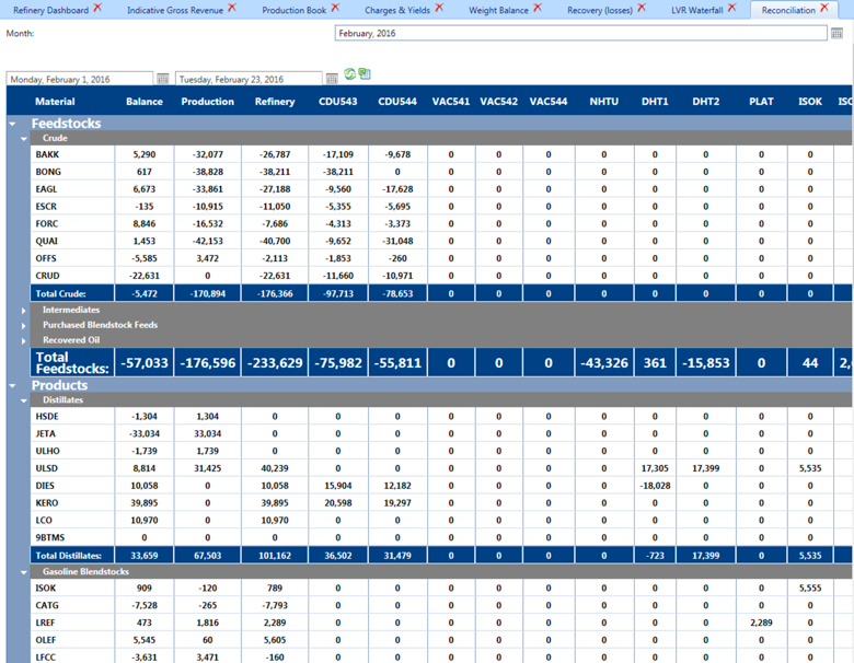
Volume Reconciliation

To access the Reconciliation display, navigate to: Dashboards> Profit & Loss KPIs > Refinery Dashboard > Indicative Gross Revenue > Reconciliation
Similarly to the Production Book, the Reconciliation display includes tables for feedstocks and finished products. The sign convention is that a production is positive and a consumption is negative. This table can assist reconciling data by volume (while STMS reconciles by weight); it present 2 set of data, and the difference between the two:

• Column "Production" shows the yield accounting information; first raw materials, then products (including intermediates)
• Column "Refinery" is the sum of all columns to its right: it represents how the various feedstocks are processed and intermediates blended,
• Column "Balance" is "Refinery" - "Production". Even for a fully weight reconciled balance, there will be volume differences remaining. This can be due to gravity errors and/or crude composition errors. PMRC enables a manual reconciliation process by which the trial balance (see below) is exported to Excel in three different sheets: Raw, Reconciled, and Difference. It shows expected LVR for each unit in the top rows. The exercise then consists of making manual changes to get all rows to show "zero" in the balance column. This exercise is much more difficult if the refinery is not fully reconciled by weight, but can be done in a few hours with knowledge of events which occurred within the selected period (which should be reflected in LPOs and action items")

The table can be exported to Excel by clicking the Export to Excel button. The excel sheet refreshes every-time there is a new export, therefore the user must save the reconciliation results under another file name if they are to be saved for reference.

Exporting to Excel creates 3 sheets: BackcastRaw, BackcastRec, and BackcastDelta. The user will utilize BackcastRec to tweak process units inputs/outputs and Blends inputs/outputs in order to zero out the column balance as shown below (in Excel format).

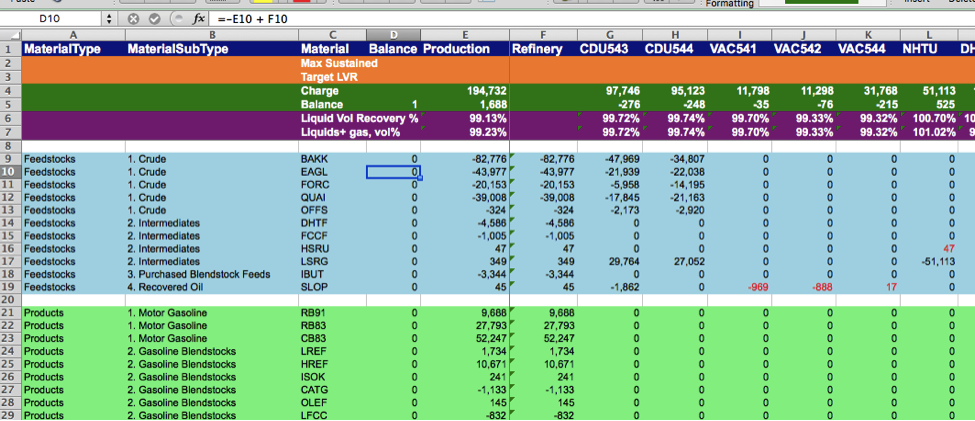
Once the user is finished, they will publish the data back to PMRC through a button placed in the Excel sheet.

Results

Summary

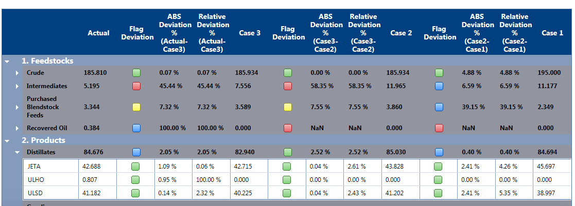
The Backcast Summary display presents a summary comparison than can be used as an executive summary for presentation purposes. It also contains one set of flags per Case difference. For the Actual - Case 3 difference, PMRC present a relative (Actual/Case3 in percentage) and an absolute difference (Actual value or percentage - Case value or percentage).

The Backcast Summary contains links to navigate to Backcast Fence-Line and Backcast Refinery displays.

At the top of each display, the user can press the Export to Excel button to export the entire dataset to an Excel worksheet that contains all the information.

Margin & Fence Line

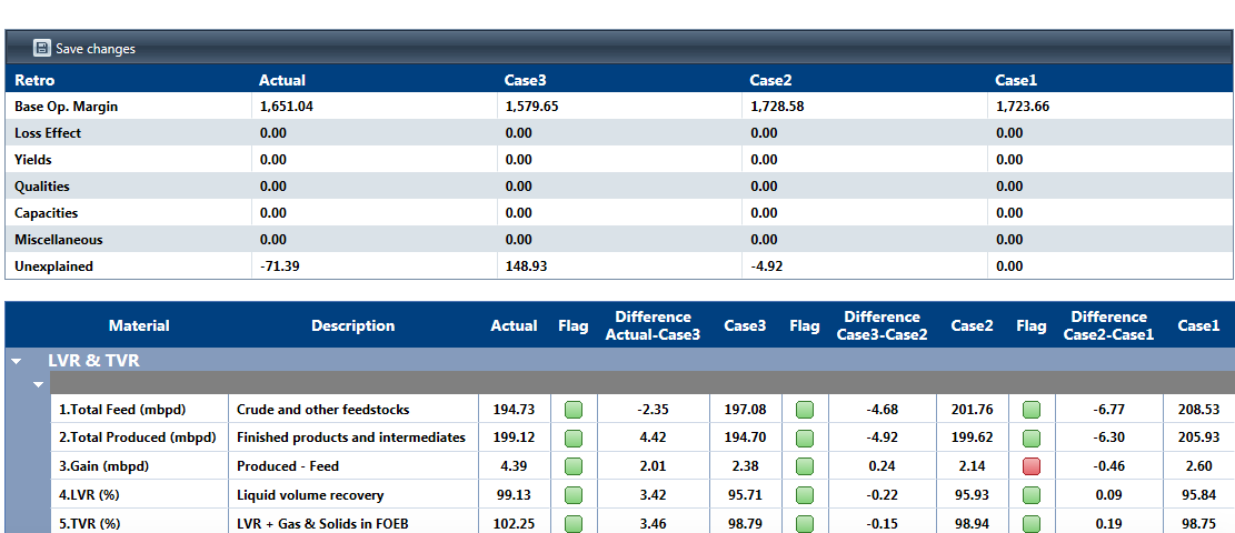
Backcast Fence Line sets up the analysis and contains section windows at the top that allow the user to define which LP case are assigned to Case 1, 2 and 3. PMRC manages the mapping between Actual and Plan systems, so it can display comparison data side by side. Users can run multiple backcast cases, load them into PMRC (through a Plan loader tool), and then decide which one is allocated to Case1, 2 and 3 for the study. Upon refreshing the screens, the base comparison will be shown for the gross margin, including key parameters such as volume recovery and crude charge. After the analysis of differences has been performed, the user can allocate the gross margin differences between: Actual and Case 3; Case 3 and Case 2; Case 2 and Case 2. The differences are displayed with four preset root causes (losses, yields, qualities, capacities) - the balance is calculated automatically.

The Displays shown below are further presenting the Case values and differences between them in terms of production/consumption rate and parameters.

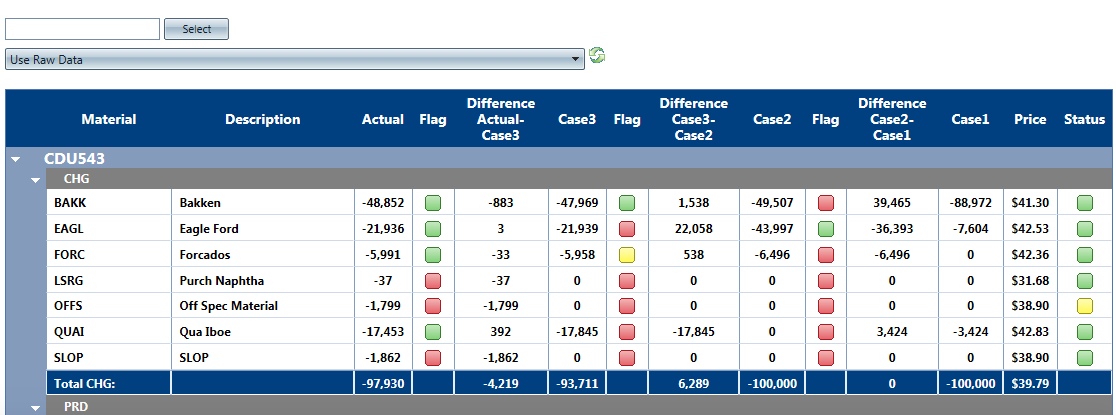
Process Units

This set of displays presents each process unit side-by-side as defined in the yield accounting system or the preloaded volume reconciled data (preferred - see Reports Folder).

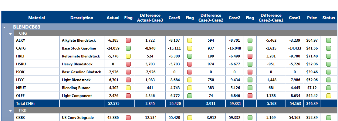
Blends

This set of displays presents each blend side-by-side as defined in the yield accounting system. Here again, the volume-reconciled information can be used instead of the original STMS data if minor changes are made in the blend columns.

Reports Folder

The reports folder is a small application that allows anybody to get to all Excel files used in the study (volume reconciliation and report). It is also where the volume-reconciled data can be uploaded for usage in the case comparisons. In order to add a "volume reconciled" file and use it as source of data for the reports, there are two choices:
From the Process Unit Menu

Click the select button, find the file on your PC and hit save.
From the reports menu:

Use the upload button to load your file.

From that point, the file is available to PMRC. The user has the choice to use it by selecting on the process unit window below.

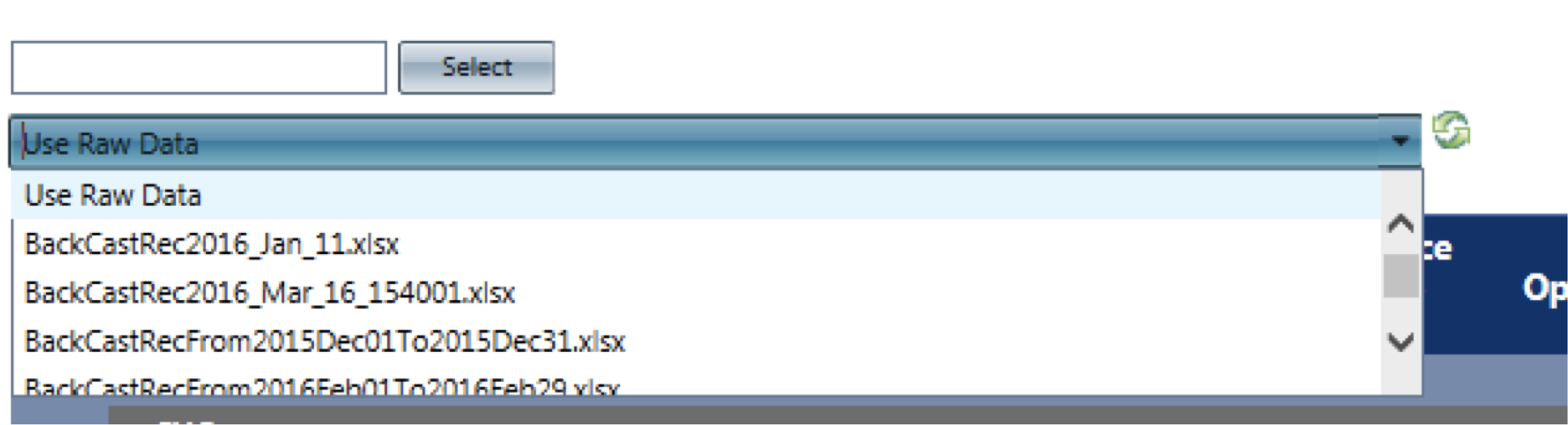
The option Use Raw Data is the default option, and it uses PMRC original data only (yield accounting based).

 

Appendix

Price and Plans Loader

PMRC requires periodic updates to production plans and to prices, both "planned" or forecast for the prompt month, and actual (current market). The intent for displays is not to reproduce accurate financial statement/gross revenue, but to give an indication on whether or not current market based prices are in line with forecast. PMRC backcast application also needs the ability to load a plan, made after the end of the month (backcast) that contains production and price information For the above, there are currently two sources of information used by PMRC, both created by the Optimization group in Atlanta:

• The pricing sheet contained in a "Dashboard" workbook, which generates "actual" benchmark based prices.
• The monthly plan reports obtained as output of the linear program Petro, which contains purchases, sales, unit charge & yields, blending information and prices/costs.

And there is one source of information similar to the monthly plan reports that is currently generated at Trainer, part of the Backcast process.

Each of those two source types is handled separately as described below.

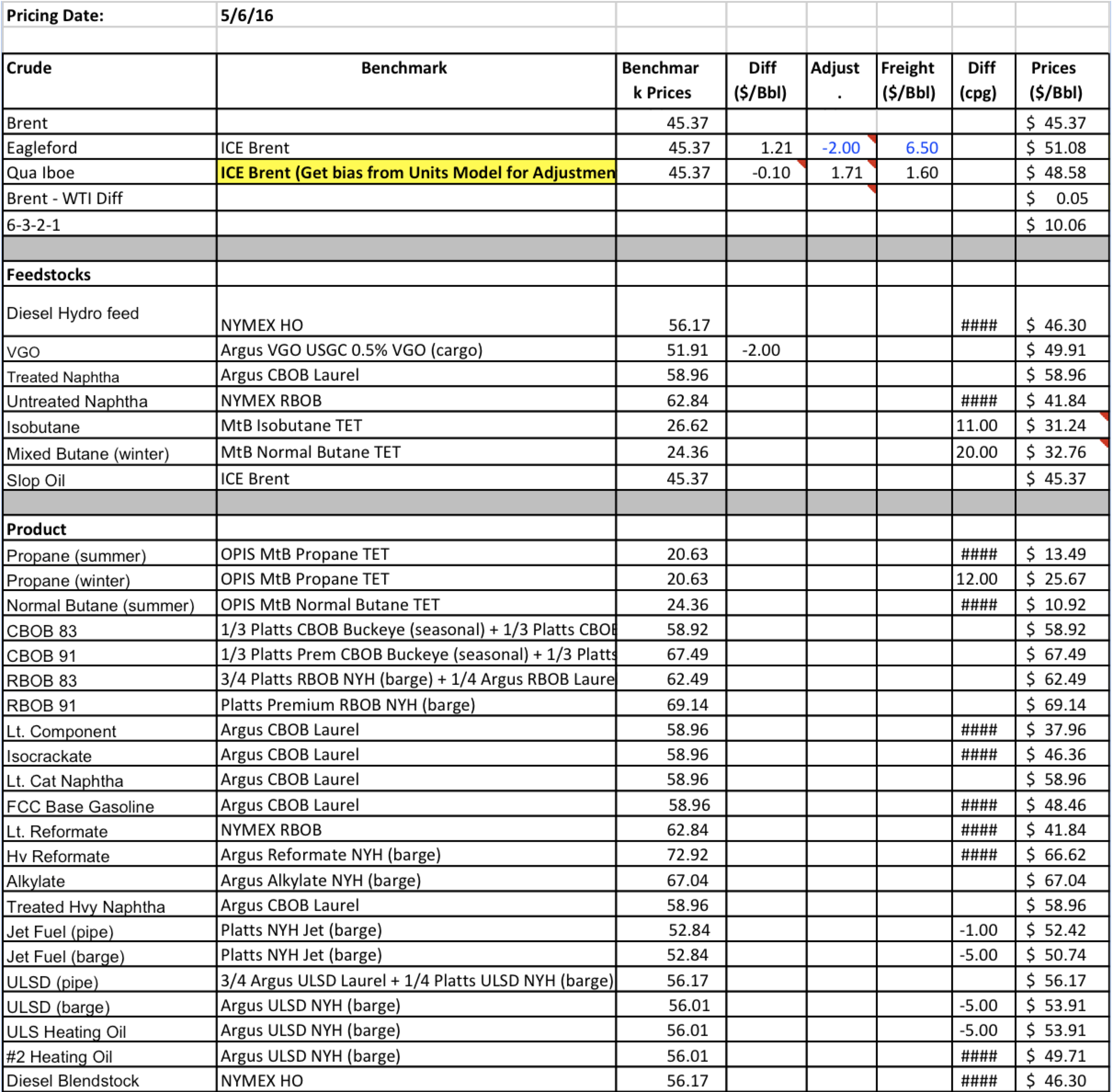
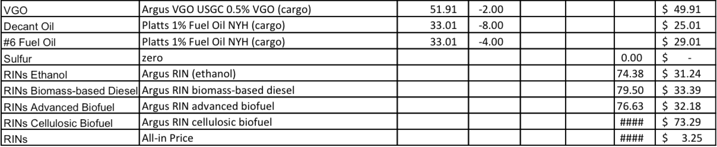
Pricing Sheet

The process is entirely automated. Every time the dashboard sheet is saved in Atlanta, a copy of the pricing sheet (see pricing sheet below) is mailed to a Trainer outlook mailbox from which is treated on an hourly time schedule to insert directly in PMRC. Contact the IT department for troubleshooting in case Actual prices do not seem to be updated. This would be noticed if Actual prices for a commodity such as CBOB83 are equal to planned prices (the PMRC logic in order to avoid any false conclusion due to lack of prices).

Monthly Plan and Backcast Output

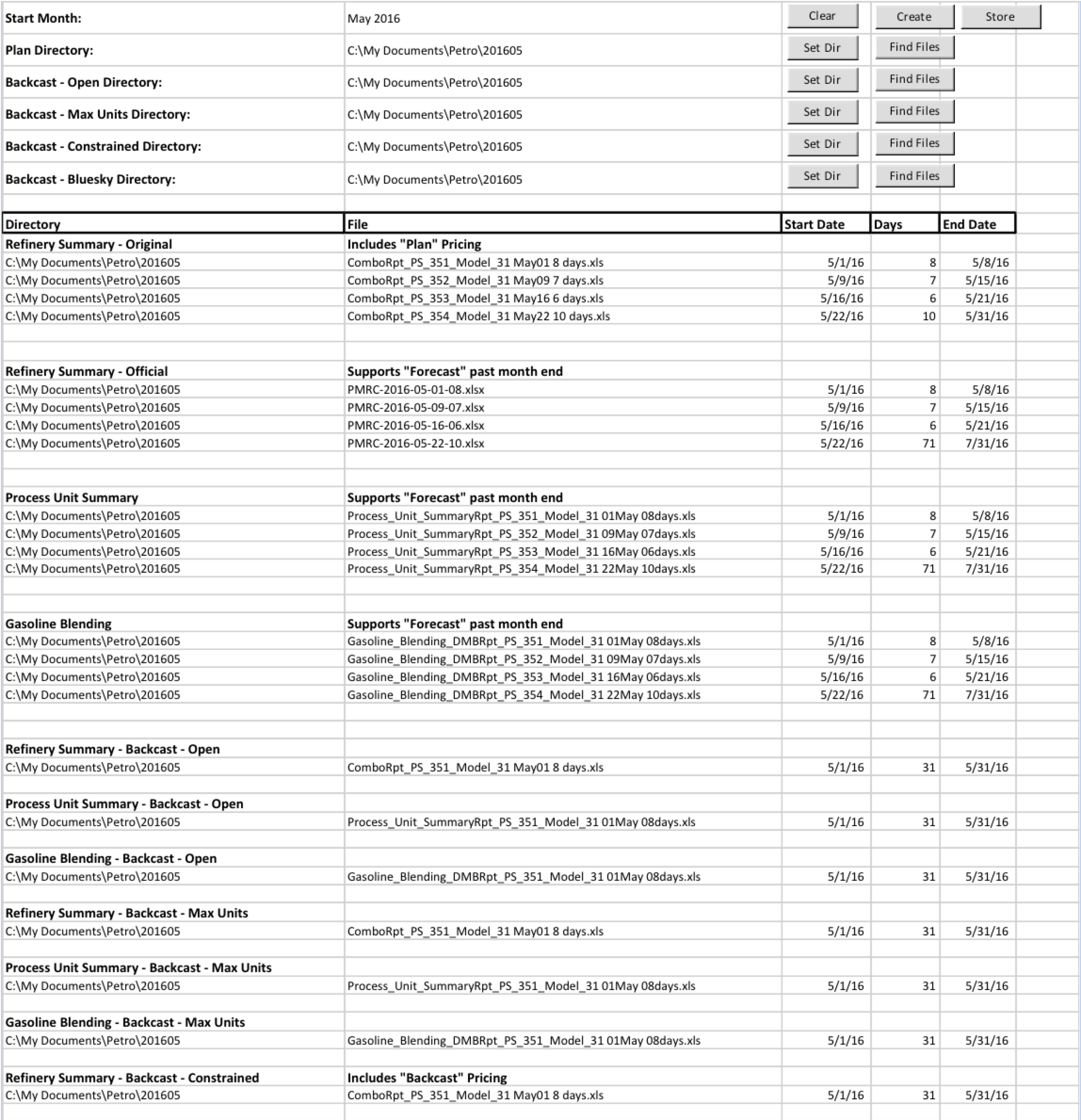
This process requires the use of a XLS based loader (see PetroPlan_DMI_Loader_xxxx below) as it involves three to four files per occurrence. The loader is available on the network under /../Planning & Economics/ Those standard files are (listed with a recommended nomenclature):

• Comborpt_Model version_start day_number of days
• Process_Unit_Summary_version_start day_number of days
• Gasoline_Blending_version_start day_number of days
• PMRC-yyyy-mm-startday_number of days

"Comborpt" contains purchases, sales and prices. "Process Unit Summary" and "Gasoline Blending" contain process unit charge and yields as well as components blended for each finished gasoline grade. The three files when associated to a planning period form the "Original" plan. PMRC is a file that allows for small edits of the purchases and sales in order to match the plant better. PMRC loads as the "official" plan but does not reconcile with process units or blends (comborpt - the Original - is reconciled with process units and blends).

Each backcast run only needs the three first files (Comborpt, process unit summary and blending) as there is no editing occurring in this case. However, we have allowed four separate cases to load at once, representing possible backcast runs (Constrained: closest to actual production; Max Units: important units at their maximum capacity, Open: more crude oil purchases and other product grades open, Blue Sky: an even less constrained model - see Backcast display for more explanations).

The process to follow is then identical whether loading plan or backcast results and can be execute by different people:

1. Request 4 files (XL) for each period in the plan to be either sent by email or loaded on the ZeoNet cloud (the current process)
2. Save files onto a specific month directory (ex: S\...\..\Plan\201605 for May plans or S:\...\..\Backcast\201605 for backcast runs for May)
3. Open the XL loader and locate the "parameter" sheet (far left)
4. Select Clear
5. Update Month in B1
6. Update Directory (typically only update the last part ex:201605 to 201606) and select "Set DiR"
7. Select "Find Files"; if the nomenclature has been followed, the file names will appear in the respective locations, line 10 to 34 for plans and below for Backcast. Note Backcast only contains one period so we expect only one line per run type and per file type.
8. Verify that all expected file names have been updated. If not (if the nomenclature does not match expected format), type the file name directly into column B and update start time and number of days (End date is a formula).
9. Select Create: this will update all Tabs in the workbook with pre-loading information. Verify each tab, column C for any sign of material mapping error ("Unmapped" would appear in the first lines before all mapped materials). A mapping error can occur if the plan contains a crude never processed for instance. In this case, contact IT to refresh the internal mapping and re-run Create.
10. When mapping issues are resolved, select "Store", In PMRC, the last plan stored or last price stored wins so multiple loading will not affect the results.

Pricing sheet: Pricing_yyyymmdd:

 

Plan Loader: PetroPlan_DMI_Loader